This page contains improvements to the AWR Design Environment for PA designers.
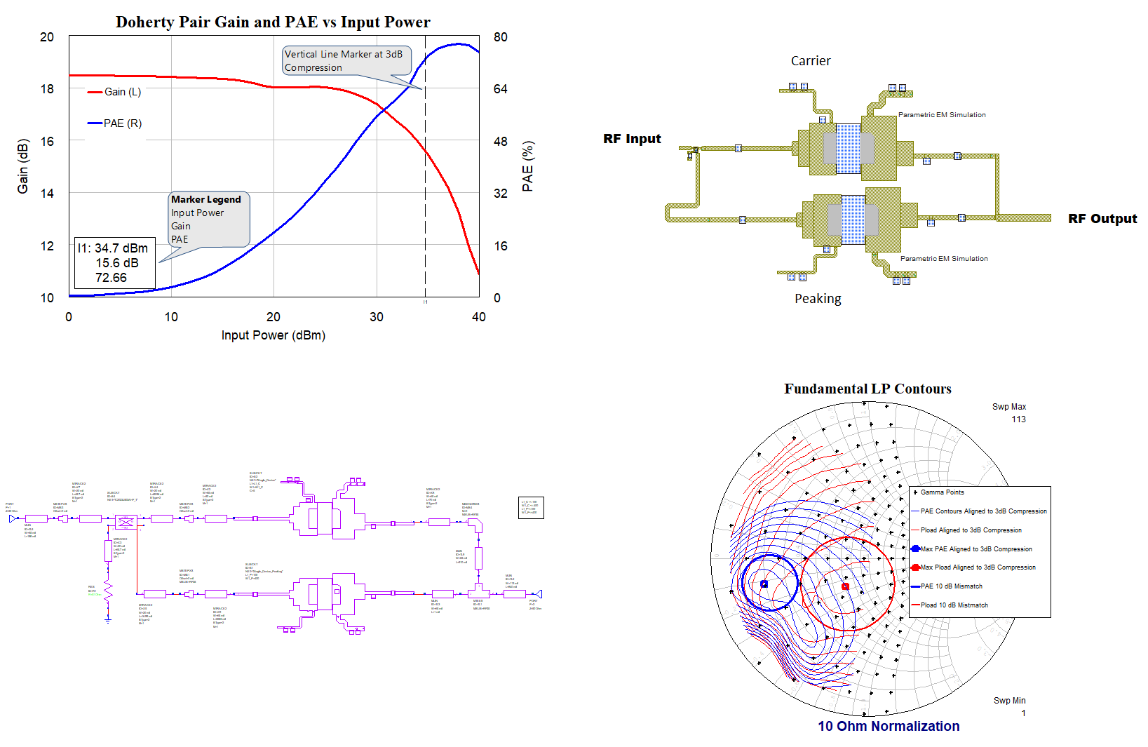
Save time with PA design flow overviews and exampleSee the Power Amplifier Design Flow Knowledgebase page for an in-depth look at this project and flow used in the design of this Doherty power amplifier. |
|
This page lists improvements to the AWR Design Environment for PA designers.
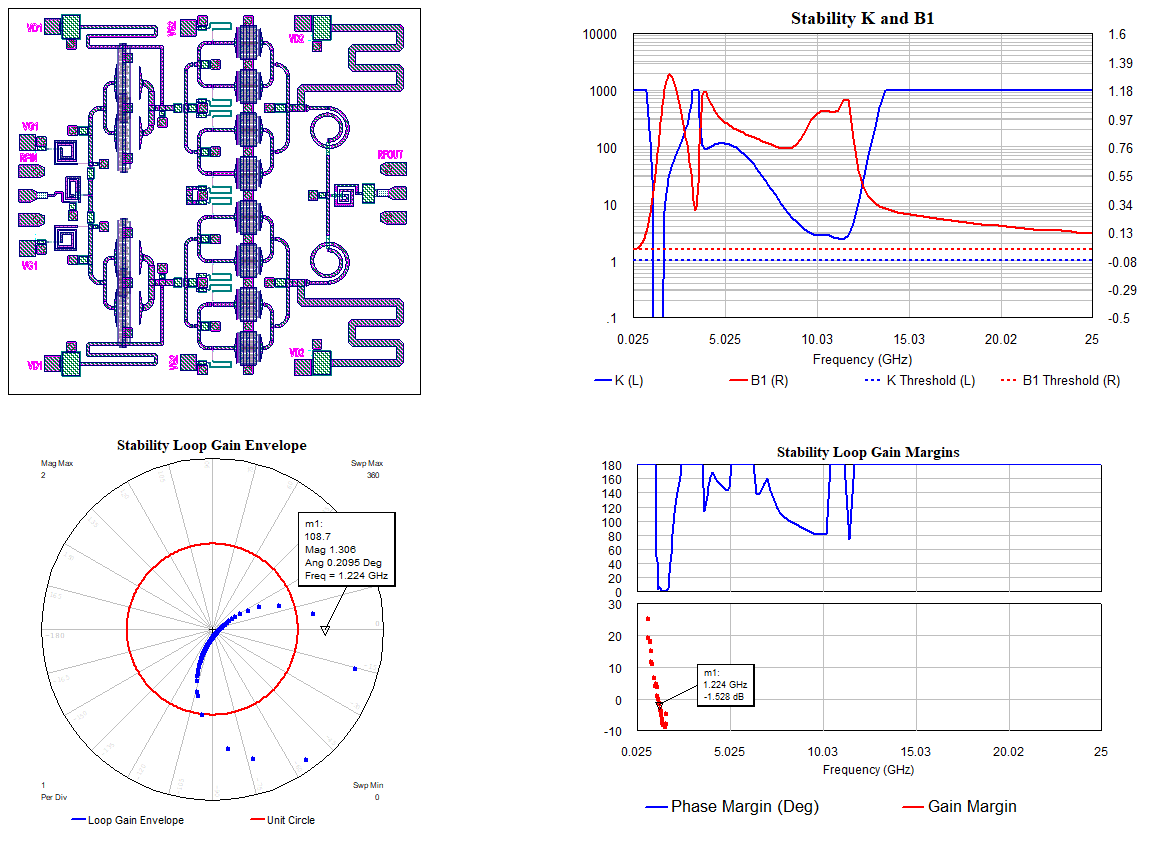
Perform Fast Linear and Nonlinear Stability Analysis Using Loop Gain Envelope EvaluationThe project opens to a data display page and simulates. License Requirements: Linear or Nonlinear Simulation and Advanced Stability Analysis (STB_100)
|
|
|
|
|
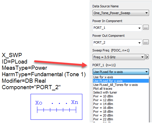
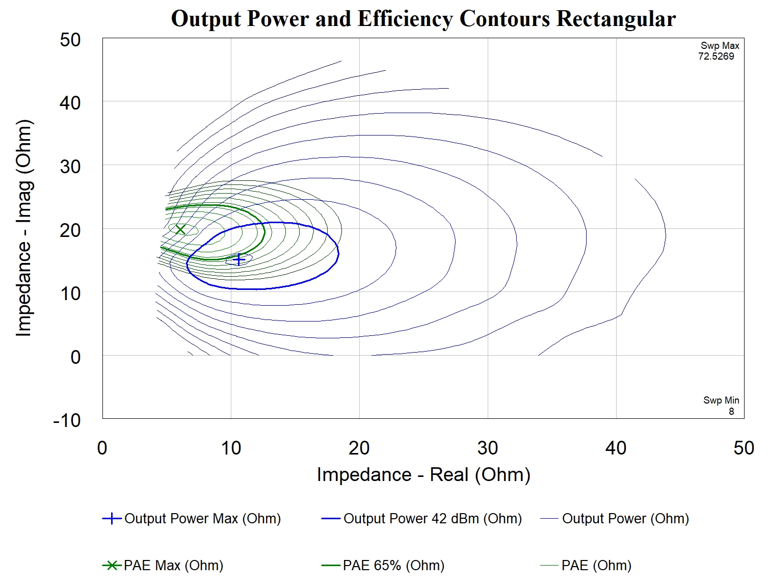
Directly Read Impedance Values from Load Pull Contours on Rectangular Real/Imaginary GraphsThe project opens to a data display page and simulates. License Requirements: Load Pull (LPL_100)
|
|
|
|
|
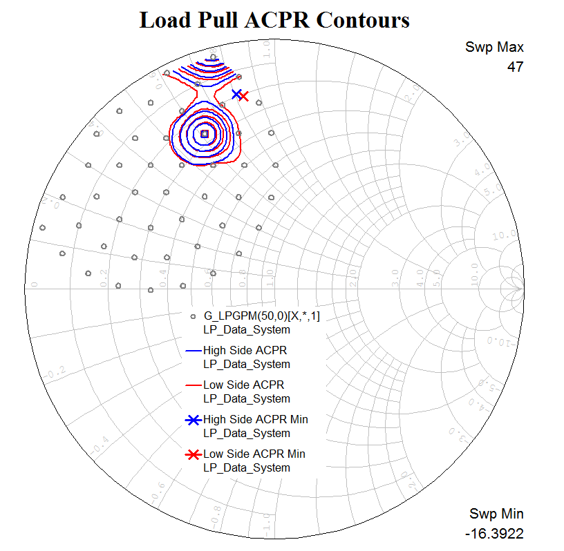
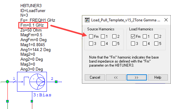
Simulate the Impact of Video Bandwidth or High-order Harmonic Impedance on PA PerformanceThe project opens to a load pull template schematic and a data display page and simulates. License Requirements: Load Pull (LPL_100)
|
|
|
|
|
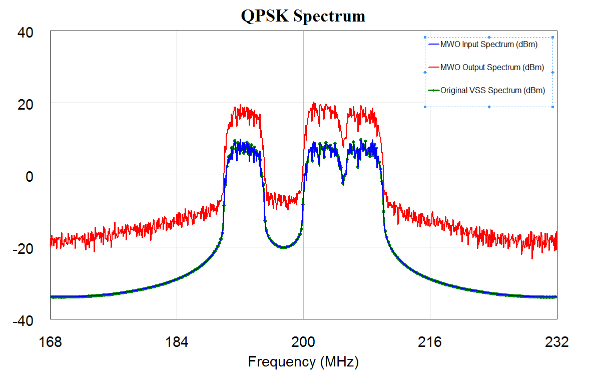
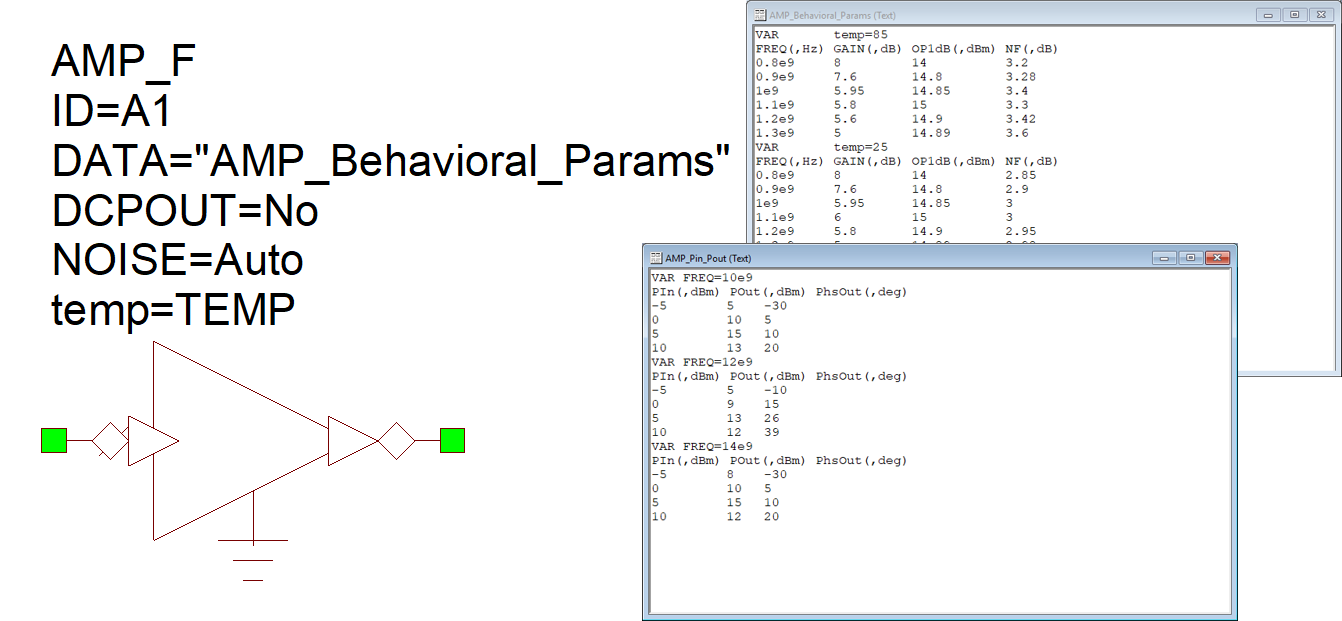
Easily Set Up PA Model ReuseThis project illustrates improvements to the AMP_F file-based amplifier, which now supports two types of data files. License Requirements: VSS Time Domain (VSS_250+)
|
|
|
|
|
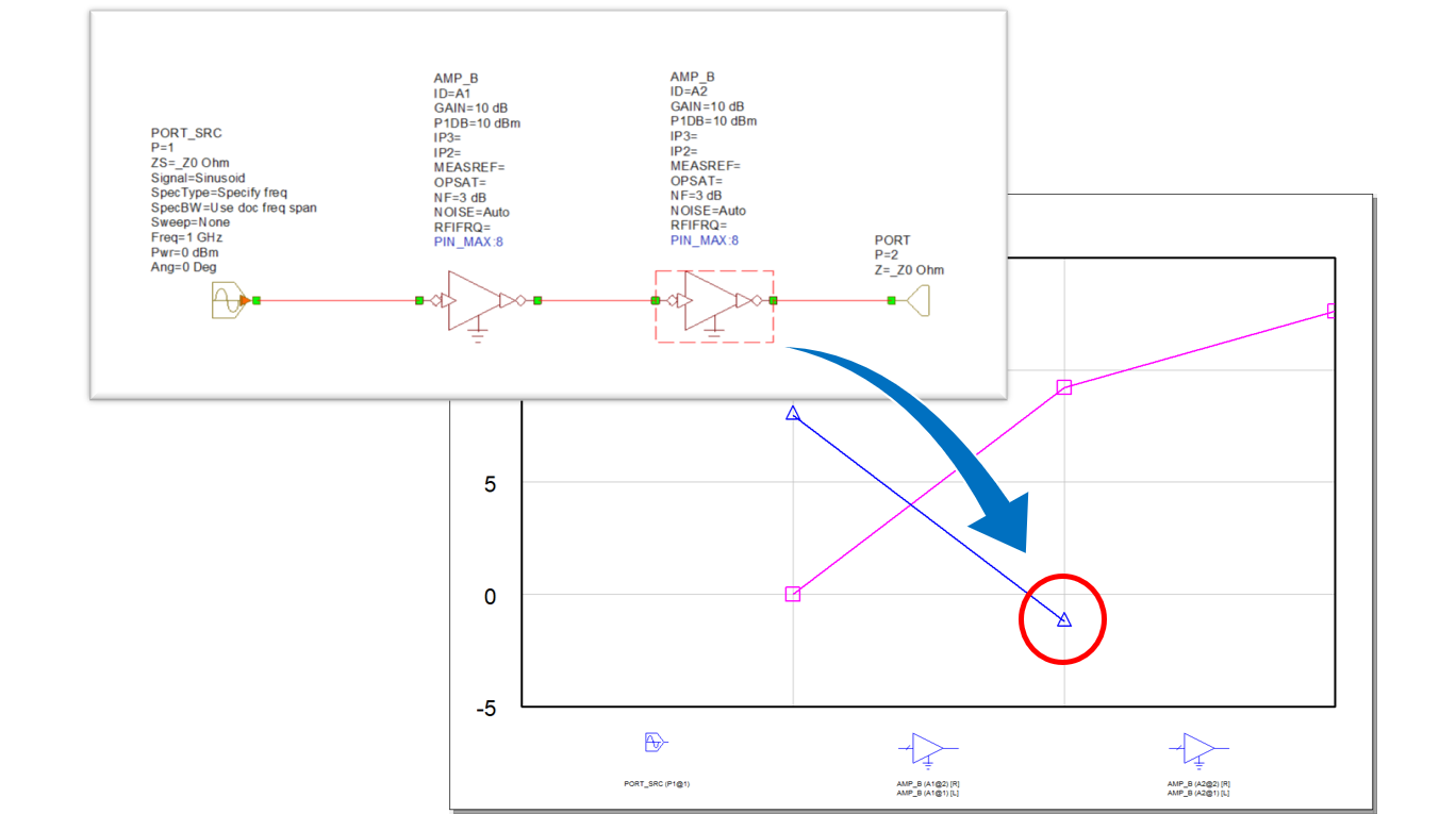
Inspect System Diagrams for Damage from Overdriving the DevicesThis project shows how to use the new cascaded damage indicator measurement, C_DAMAGE, in VSS. License Requirements: VSS RF Budget (VSS_150+)
|
|
|
|
|
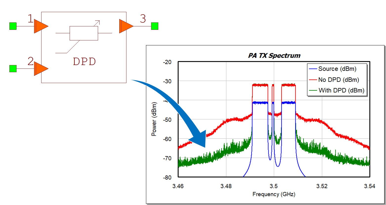
Evaluate Device Linearization before Building it? / Test Drive Classic or Commercial DPD Algorithms?This example illustrates linearization of a PA using the new DPD block in VSS. License Requirements: VSS Time Domain (VSS_250+)
|
|
This page contains improvements to the AWR Design Environment for PA designers.
|
|
|
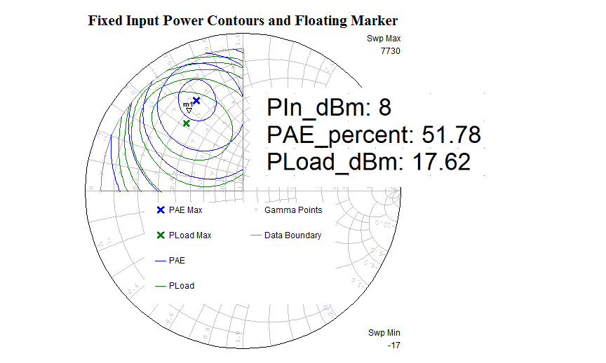
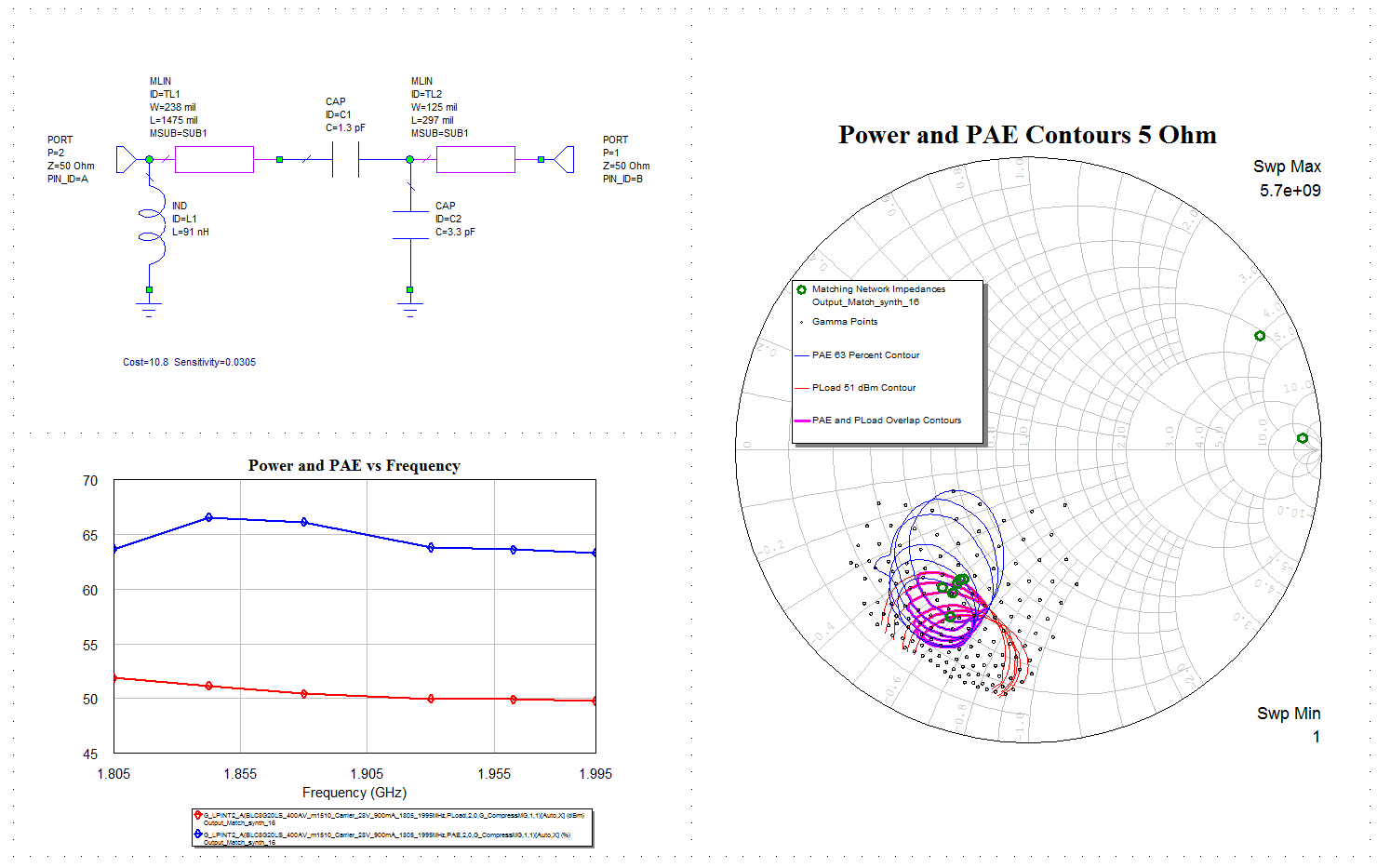
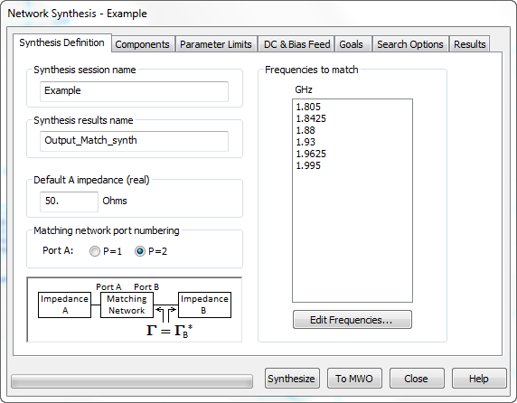
Matching Network Wizard OverviewThe Network Synthesis Wizard allows the user to specify goals and components to generate matching network topologies in a matter of minutes. In this example a PA matching network is designed to meet both PAE and output power at a fixed compression point goals. |
|
|
|
Additional Network Synthesis Wizard examples can be found on the antenna and design flow pages. The project will open to show the Matching Network Report Output Equations page and simulate. License requirements: Network Synthesis (SWS-100)
|
|
|
|
|
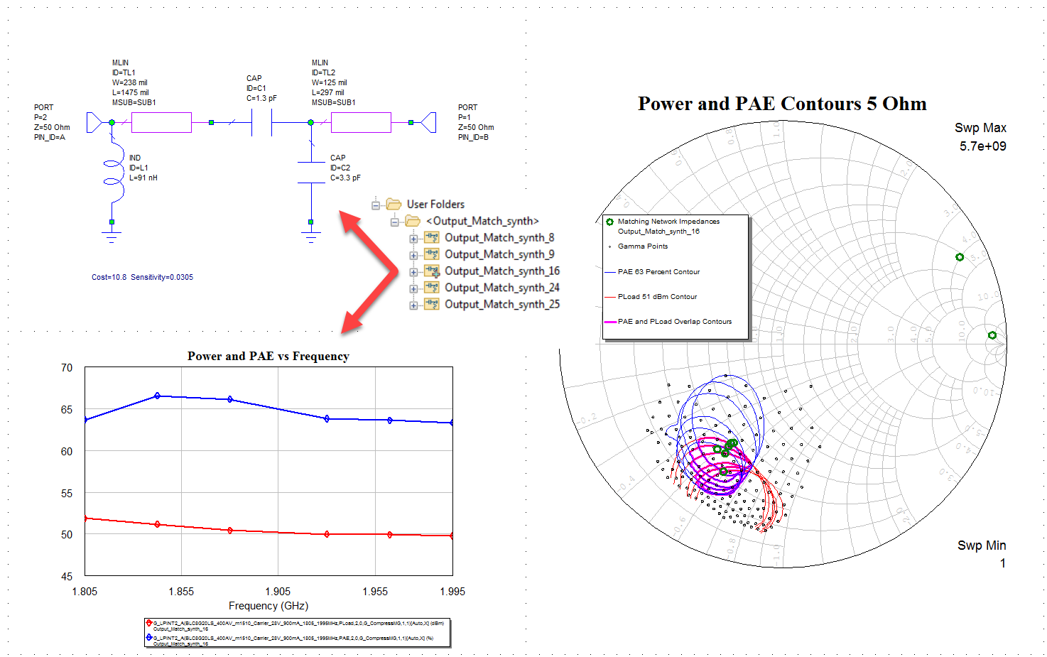
Synthesizing and sending results to Microwave Office
|

|
|
|
|
Exploring results
|
|
This page contains improvements to the AWR Design Environment for PA designers.