This page contains improvements to the AWR Design Environment for PA designers.
Create reusable data display pages for simulated and measured data.
Load Pull Reports
The project will open to the Load Pull Report Output Equation page and simulate.
Change multiple Measurement data sources with a few clicks.
Double-click on the DOC_SET element to enter edit mode
Uncheck the Sample_SPL data file and check Sample_AB data file
Click OK and note that all the Graphs update to reflect the new data source
Change multiple Measurements to plot multiple sources with a few clicks.
Double-click on the DOC_SET element to enter edit mode
Check both the Sample_SPL data file and Sample_AB data file
Click OK and note that all the graphs update to show the results from both data sources
Reset to plotting data from a single source.
Double-click on the DOC_SET element to enter edit mode and uncheck the Sample_AB data file.
Using variables in measurements
Double-click on the first measurement on the PAE and Output Power Contours at xdB Compressed graph and note that the data is aligned to the equation xdB compressed rather than specified with a number
Tune (F9) on the xdB equation
Note that the contours and displayed gamma points update accordingly as the aligned gain compression changes.
Tune (F9) on the Z0_Re and Z0_Im equations
Note that the normalization impedance for both Smith Charts change.
Interpolate load pull data using floating markers on the Smith Chart.
Floating Load Pull Markers
The project will open to show the Load Pull at Fixed Input Power Output Equation page and simulate.
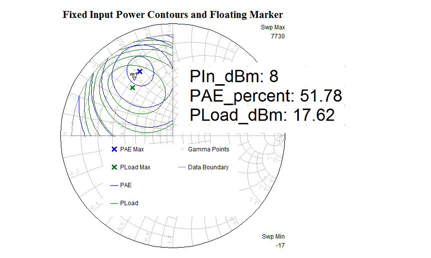
Note that the current input power is displayed as a red vertical line on the rectangular graph
Double-click on the Smith Chart to activate the view and drag m1 to select an impedance
Note that as m1 is changed the PAE and PLoad at the m1 impedance are displayed to the right of the Smith Chart under Results
The rectangular graph shows PAE and PLoad vs. input power at the m1 impedance
Tune on PIn_Tuner in the tuner to change the input power at which the contours are plotted
If desired explore the Load Pull at Fixed Compression Report Output Equations document which shows a similar setup but at a fixed compression point rather than a fixed input power
Effortlessly plot any measurement vs. output power.
Plotting vs. Output Power with X_SWP
The demo opens the project, maximizes an Output Equations page, simulates
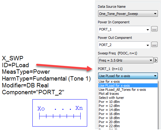
Note the X_SWP blocks on the schematic that allow the user to specify what to plot (power, voltage, current), how to measure it (spectrum analyzer style, power meter style, etc.) and where to measure it.
Double-click one of the Graphs to activate the view.
Right-click on the blue trace measurement in the legend, choose Modify Measurement and note that it uses the old PlotVs measurement that requires one measurement definition for the x-axis and one measurement definition for the y-axis.
Right-click on the red trace measurement in the legend, choose Modify Measurement, and note that it is a "normal" measurement for which you can plot vs. output power by choosing the appropriate X_SWP_ID in the PORT_1 sweep drop down.
If desired, inspect all the graphs in the Report One Tone and Report Two Tone Output Equation pages to explore different X_SWP configurations.
Jump-start matching network design using the Network Synthesis Wizard.
Matching Network Wizard Overview
The Network Synthesis Wizard allows the user to specify goals and components to generate matching network topologies in a matter of minutes. In this example a PA matching network is designed to meet both PAE and output power at a fixed compression point goals.
Additional Network Synthesis Wizard examples can be found on the antenna and design flow pages.
The project will open to show the Matching Network Report Output Equations page and simulate.
License requirements: Network Synthesis (SWS-100)
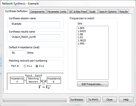
Open the Example instance of the Network Synthesis Wizard and review the setup on each tab
Synthesis Definition - defines the "direction" of the matching network and frequency band(s) of interest.
Components - defines the available series and shunt components as well as first component and last component limitations.
Parameter Limits - defines the parameter limits, parameter rounding, component series, etc. for each component.
Note that the L and C are limited to the E24 value table and that the MLIN values round to 1 mil.
DC & Bias Feed - defines the matching network DC path constraints and the bias injection network that the wizard should consider.
Note that because this is a PA output matching network Port B must be a DC open to ground
Goals - defines the Measurements and Goals for the synthesis. Double-click on a Measurement or Goal to see the setup.
Note that the examples in this measurement use the load pull data as the source and define PAE and Output Power at 1 dB Compressed.
The goals are set up for a PAE >= 63%, an Output Power >= 51 dBm, and a 2nd and 3rd harmonic region.
Select the HarmAreaMatch goal and then push the View Region button to see the specified harmonic region.
Search Options - defines advanced search options.
Results - shows the results from the Synthesis run and controls how many network and what additional data is sent back to Microwave Office.
Synthesizing and sending results to Microwave Office
NOTE: This synthesis takes a few minutes to run so there are results already saved in the project. However, if interested, push the Synthesize button to start a new synthesis. Otherwise skip to the next step to use the already synthesized results.
If you'd like to see an example that synthesizes more quickly check out the example on the design flow page.
When the synthesis is complete (or if you skipped the synthesis step) push the To MWO button to send the results to Microwave Office.
Push the OK button on the "Overwrite Options" dialog.
Push the Close button to close the Wizard.
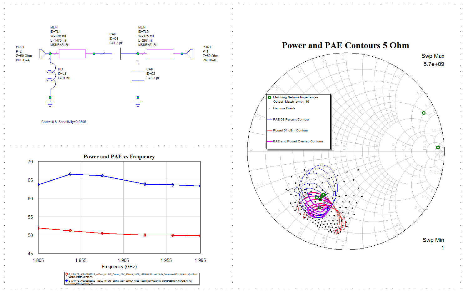
Exploring results
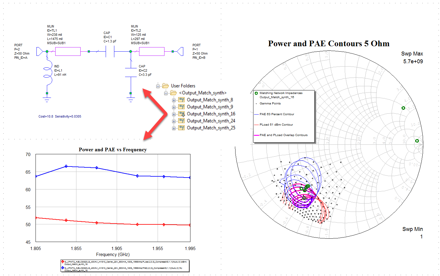
All of the generated networks have been sent to Microwave Office and placed in the <Output_Match_synth> User Folder in the Project Tree.
Click on the individual networks under the User Folder to see the results from the networks.
Note that the graph results update to show response with the selected network and the displayed schematic updates to show the selected networks